Ray Sampling

download HDA and examples

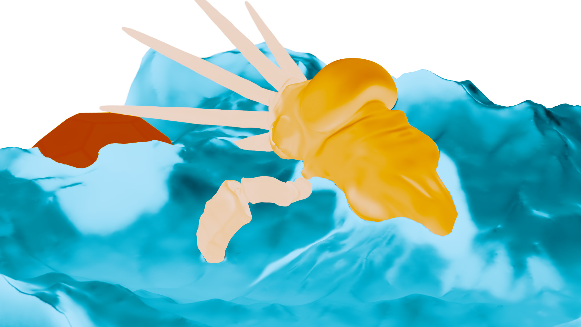
Procedural setups can gain a lot of plausibility when they use some kind of shape analysis as starting point. Lately I’ve been playing around with bullet again and thought it would be sweet to measure an objects thickness as a baseline for fracturing, like using it’s gradient to define crack lines etc. Naturally this took me on a dozen tangents but the result is a useful hda and this post.

Gathering radiance with ray sampling

Thickness
Analyzing a surface for is local thickness is pretty simple – just shoot a ray along the inverse normal on every surface point. Maybe also add a small bias to the sample position to make sure the rays don’t start directly on the surface.

//Parameters
float bias = chf("bias");
int do_reverse = chi("reverse_rays");
float maxdist = chf("maxdist");
//Variables
vector _P = v@P;
vector _dir = normalize(v@N);
float _dist = 0.0;
vector hit_P;
float hit_u, hit_v;
if(do_reverse==1) {
    _dir *= -1;
}
_dir *= maxdist;
vector off = bias*_dir;
int hit = intersect(0, _P+off, _dir, hit_P, hit_u, hit_v);
if(hit!=-1) {
    _dist = distance(hit_P, _P);
} else {
    _dist = maxdist;
}
//normalize distance
f@distance = _dist/maxdist;

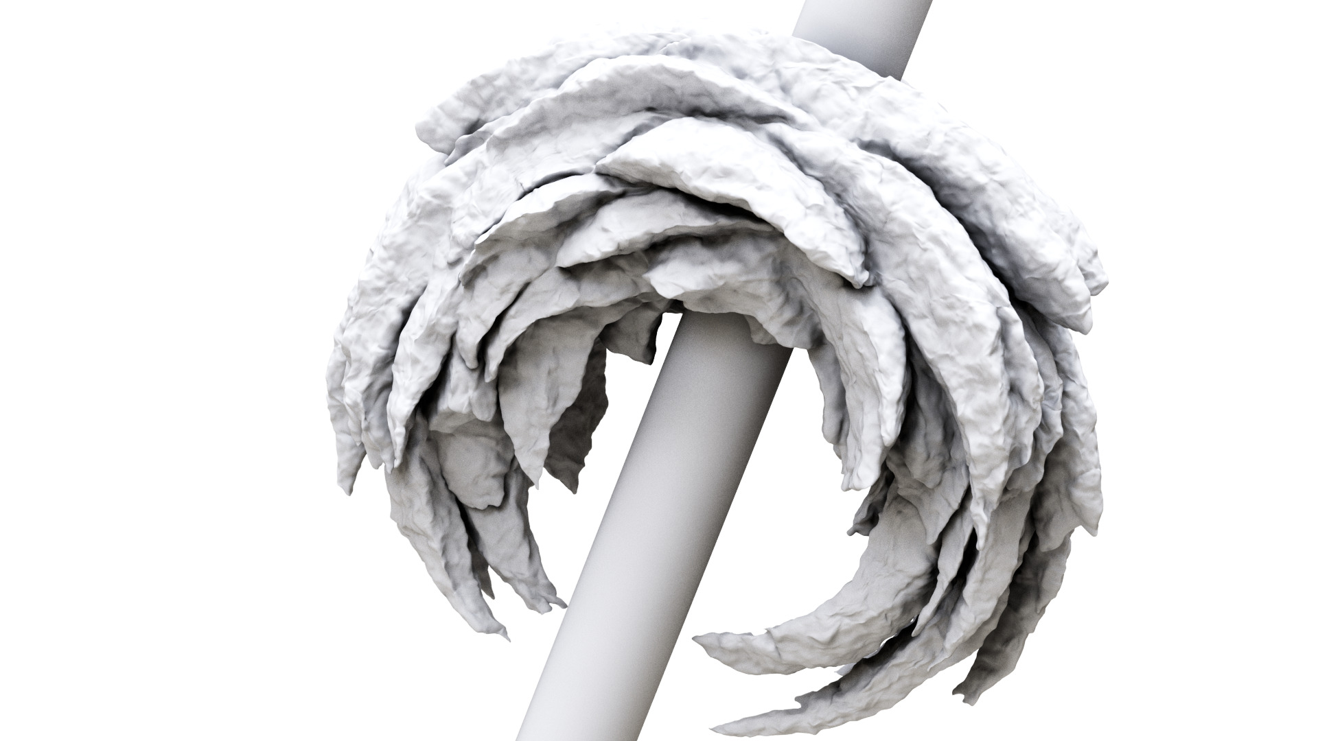
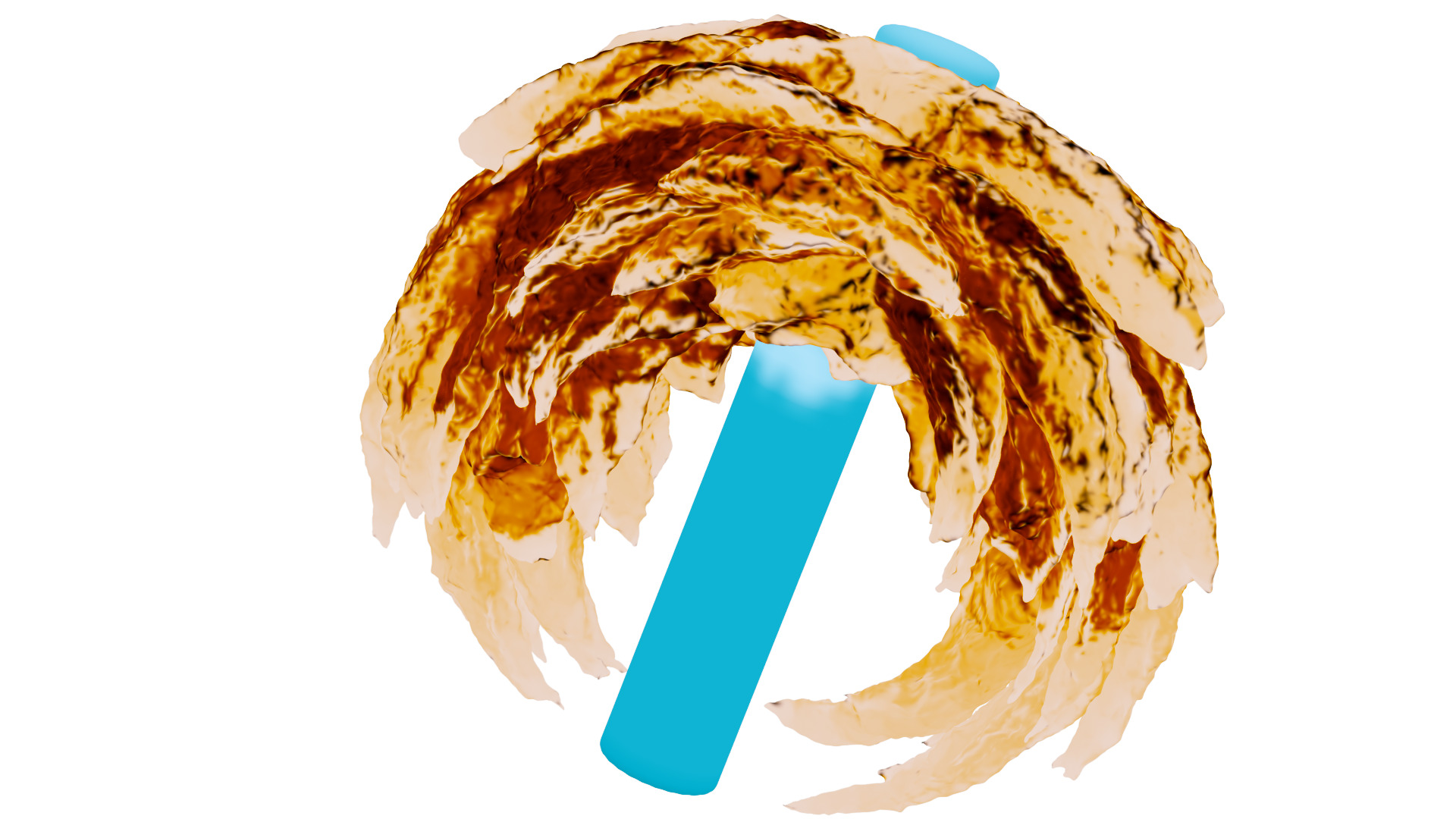
Spherical Sampling
The result is pretty crude, but it’s only taking a single sample per point. A more accurate portrayal of the points sourroundings can be obtained by taking successive random samples deviating from the normal into account.
To do so, let’s define a function which returns a ray that randomly deviates from the normal within a solid angle. The opening angle, or spread, can be exposed as a parameter: 1.0 represents hemispherical sampling, everything below is directional/glossy. 2.0 would result in full spherical sampling.

vector sampleSpherical(vector _dir, rdm; float spread;) {
    float theta = fit(rdm.x, 0.0, 1.0, 0, spread);
    float phi = fit(rdm.y, 0.0, 1.0, 0, 2*$PI);
    float _x = sin(theta)*cos(phi);
    float _y = sin(theta)*sin(phi);
    float _z = cos(theta);
    //transform sample up vector to normal via dihedral
    vector P_sph = qrotate(dihedral({0,0,1}, _dir), normalize(set(_x, _y, _z)));
    return(P_sph);
}

And wrap that into a loop that evaluates and collects the samples. Generating a unique seed per sample required some tweaking, if seeds repeat between neighbouring points the sampling pattern causes streaking artifacts.

//Variables
vector _P = v@P;
vector _dir = normalize(v@N);
vector _vattr = set(0);
float _fattr = 0.0;
float _dist = 0.0;
vector hit_P;
float hit_u, hit_v;
int hit, s;
while(s<max_samples) {
    //first sample along normal
    if(s==0) {
        dir = normalize(_dir);
    //random sampling direction
    } else {
        rdm = rand(((@ptnum+1)*(s+1))+seed);
        rdm = sampleSpherical(_dir, rdm, spread);
        dir = normalize(rdm);
    }
    dir *= maxdist;
    hit = intersect(0, _P+ off, dir, hit_P, hit_u, hit_v);
    if(hit!=-1) {
        _dist += distance(hit_P, _P);
    } else {
        _dist += maxdist;
    }
    s++;
}
//divide result by sample amount
_dist /= s;

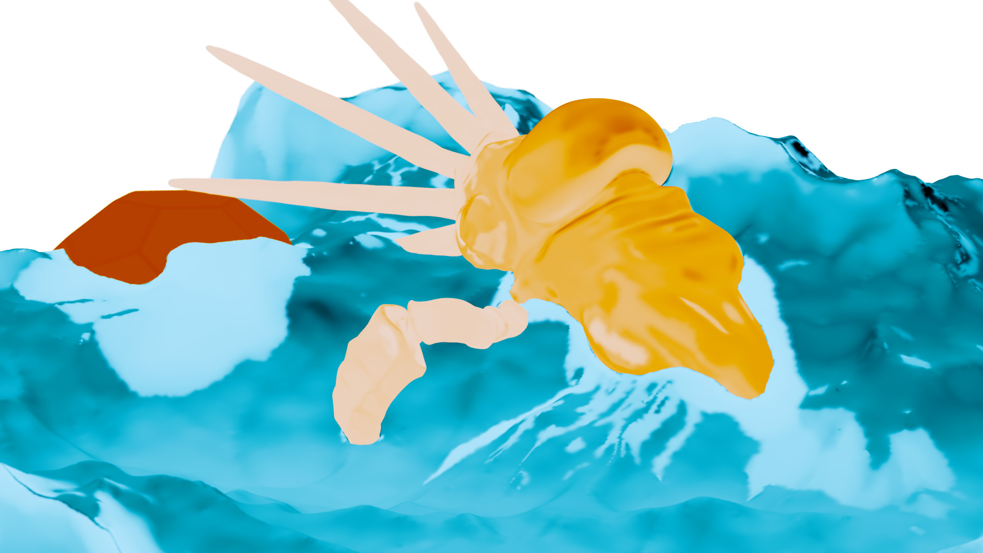
And if we don’t reverse the normal, thickness becomes ambient occlusion (outside distance)

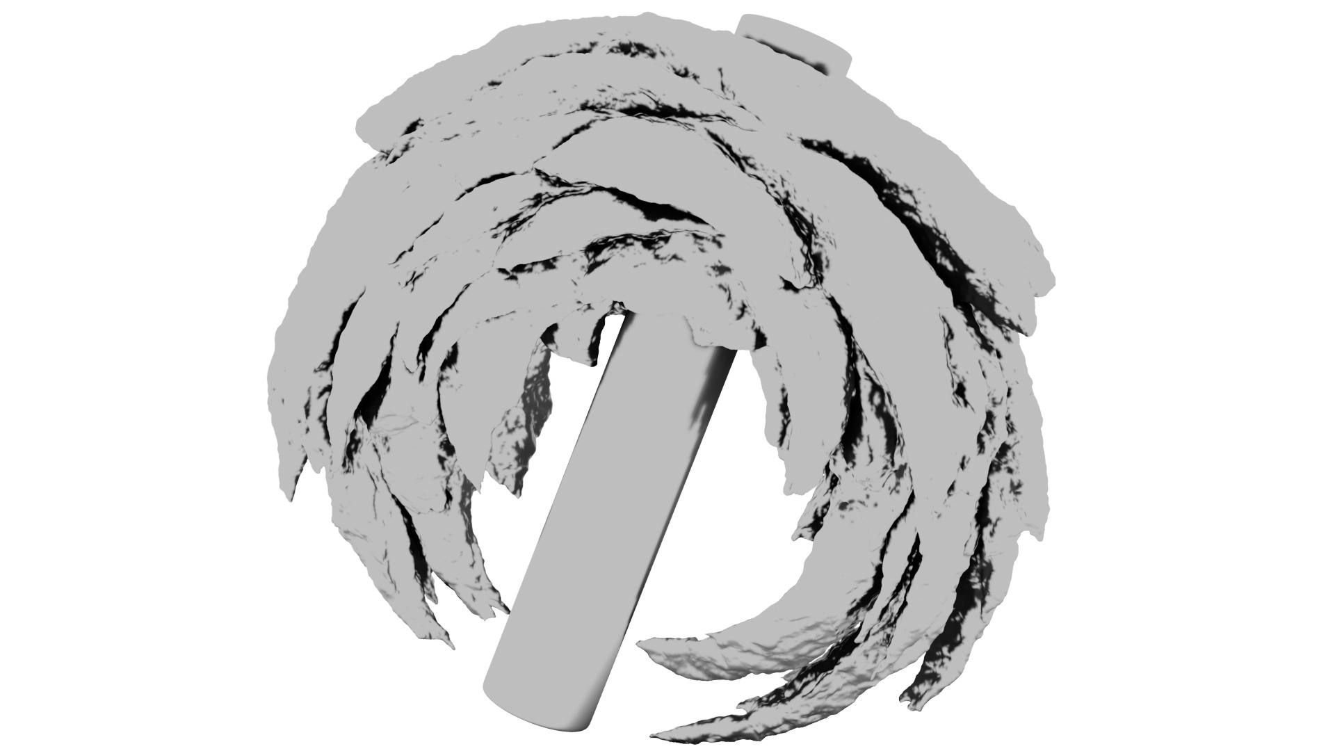
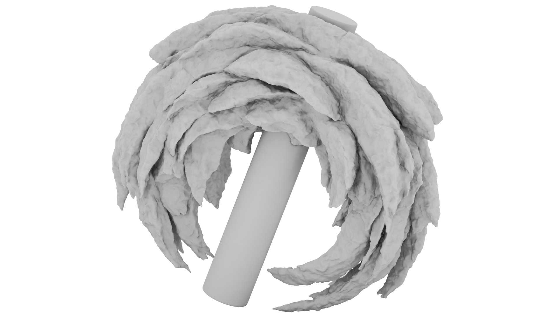
In SOP’s it can be handy for environments (scattering), polyReduce, mesh deformation….

Optimize spread
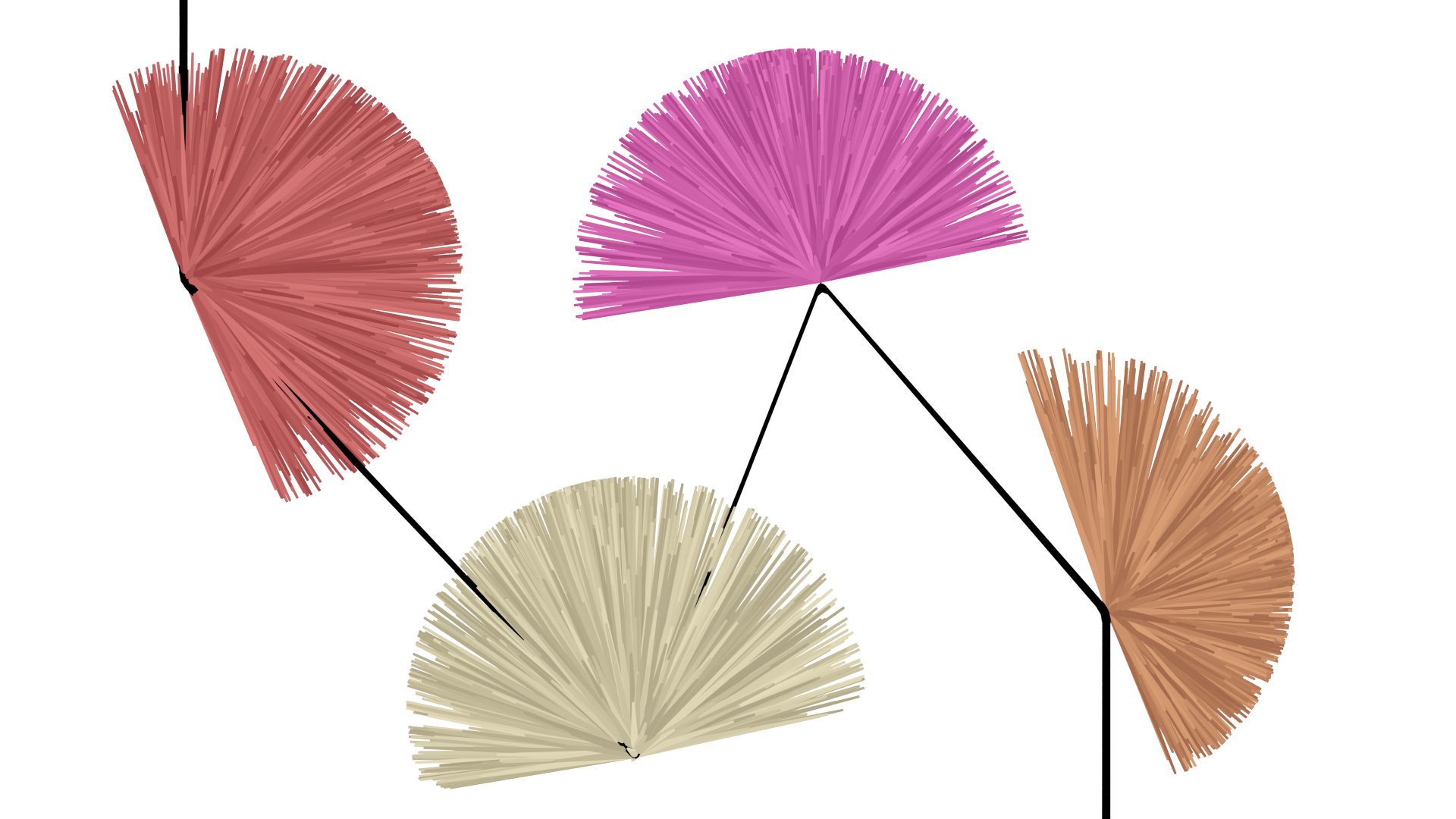
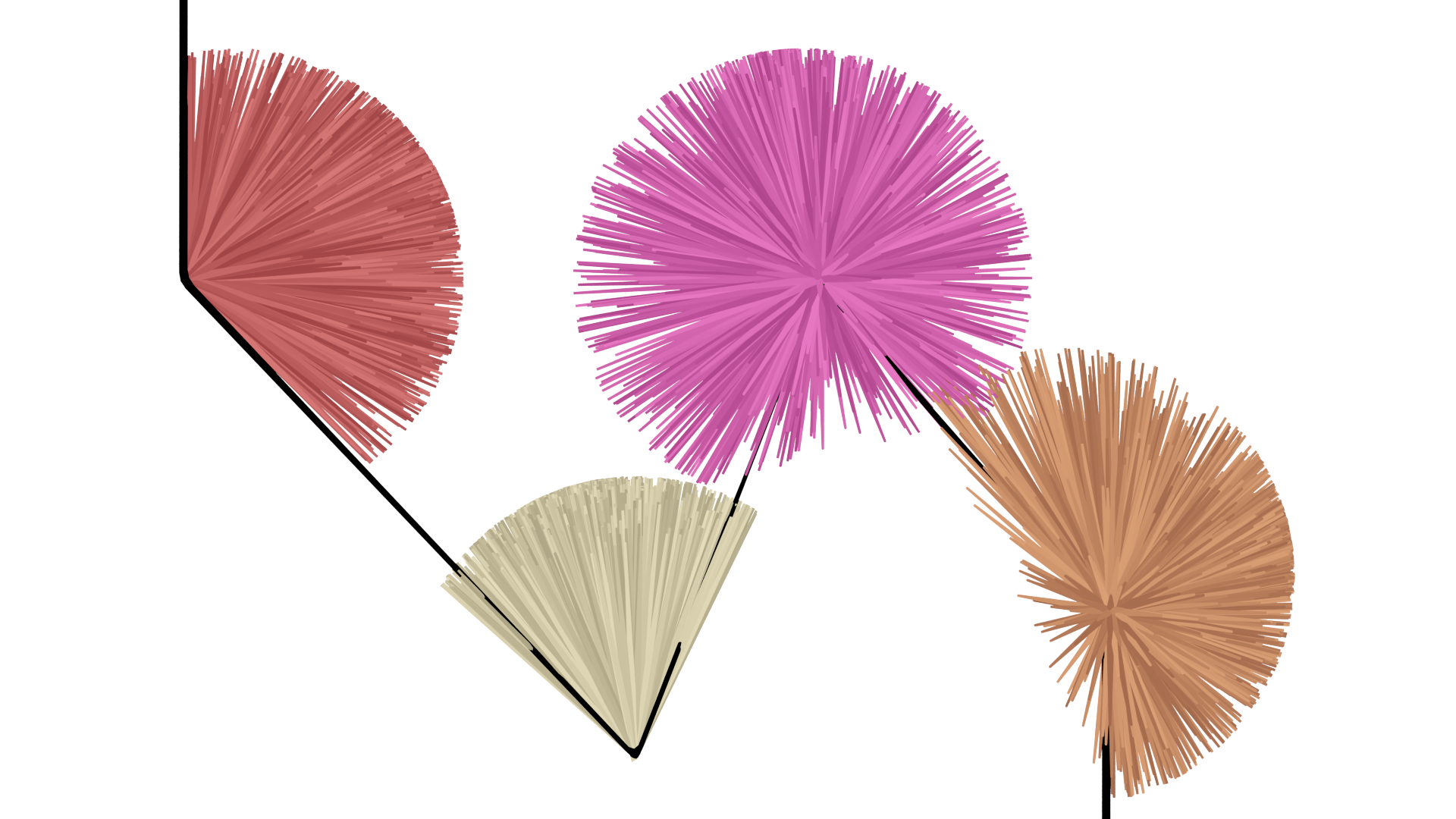
Now this is all random, no importance sampling or other bias used. Hence lots of samples are necessary for a clean result. We can at least optimize the spread angle and focus it to the local curvature of every point. By accumulating the dot product between the normal and the direction to each connected neighbour point the local ‘field of view’ or ‘fraction of visible hemisphere’ can be estimated. The spread angle in radians can be derived from that.

//Calculate curvature for spread
int crvmode = chi("spreadbycrv"); //toggle spread optimization
if(crvmode==1) {
    int neighs[] = neighbours(0, @ptnum);
    vector P_dir, P_diff;
    float accum_dot = 0.0;
    float _curvature = 0.0;
    foreach(int n; neighs) {
        P_dir = point(0, "P", n);
        P_diff = P_dir-_P;
        accum_dot += dot(_dir, normalize(P_diff));
    }
    if(len(neighs)>0) {
        accum_dot /= len(neighs);
        _curvature = acos(accum_dot)*2.0-$PI*0.5;
    }
    f@curvature=_curvature*2.0;
    if(do_reverse==1) {
        _curvature = ($PI-_curvature);
    }
    spread *= _curvature;

} else {
    spread *= $PI*0.5; //scale 0-1 spread param to radians
}

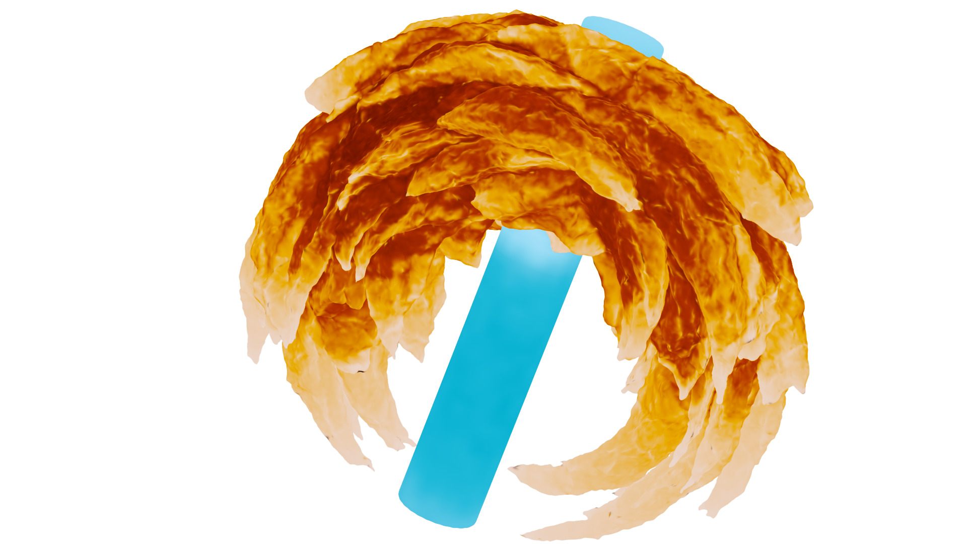
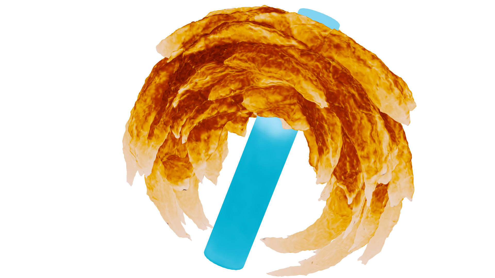
Same amount of samples, nice! Finally we may also blur the result – the normalized distance can be used as a weight attribute. And now it’s done! But wait – now that we got this ray shooter, what if….

Attributes
since we’re doing the heavy intersection stuff anyways we might as well use the hit data it returns to look up an attribute on the collision surface. So, inside the collection loop:

string attrib = chs("attrib");
int attrib_mode = chi("operation");
//0 - int, 1 - float, 2-float2, 3-vec, 4-vec4
int attrtype = attribtype(0, "point", attrib)*attribsize(0, "point", attrib);
int do_attrdist = chi("scale_by_distance");
int do_attrangle = chi("scale_by_incidenceangle");

float _fattr; 
vector _vattr;
//inside the sampling loop
if(do_attrib==1) {
    if(do_attrdist==1) {
        distWgt = chramp("distWgt", fit(dist_curr, 0.0, maxdist, 0.0, 1.0));
    }
    if(do_attrangle==1) {
        vector N_sample =  primuv(collider, "N", hit, set(hit_u, hit_v, 0.0));
        incWgt = chramp("angleWgt", fit(dot(normalize(v@N), normalize(N_sample)),-1.0, 1.0, 0.0, 1.0));
    }
    //float type
    if(attrtype==1) {
        float __fattr = primuv(collider, attrib, hit, set(hit_u, hit_v, 0.0));
        if(do_attrdist==1) {
            __fattr *= distWgt;
        }
        if(do_attrangle==1) {
            __fattr *= incWgt;
        }
        _fattr += __fattr;
    //vector type
    } else if (attrtype==3) {
        vector __vattr = primuv(collider, attrib, hit, set(hit_u, hit_v, 0.0));
    if(do_attrdist==1) {
        __vattr *= set(distWgt);
    }
    if(do_attrangle==1) {
        __vattr *= set(incWgt);
    }
    _vattr += __vattr;
}

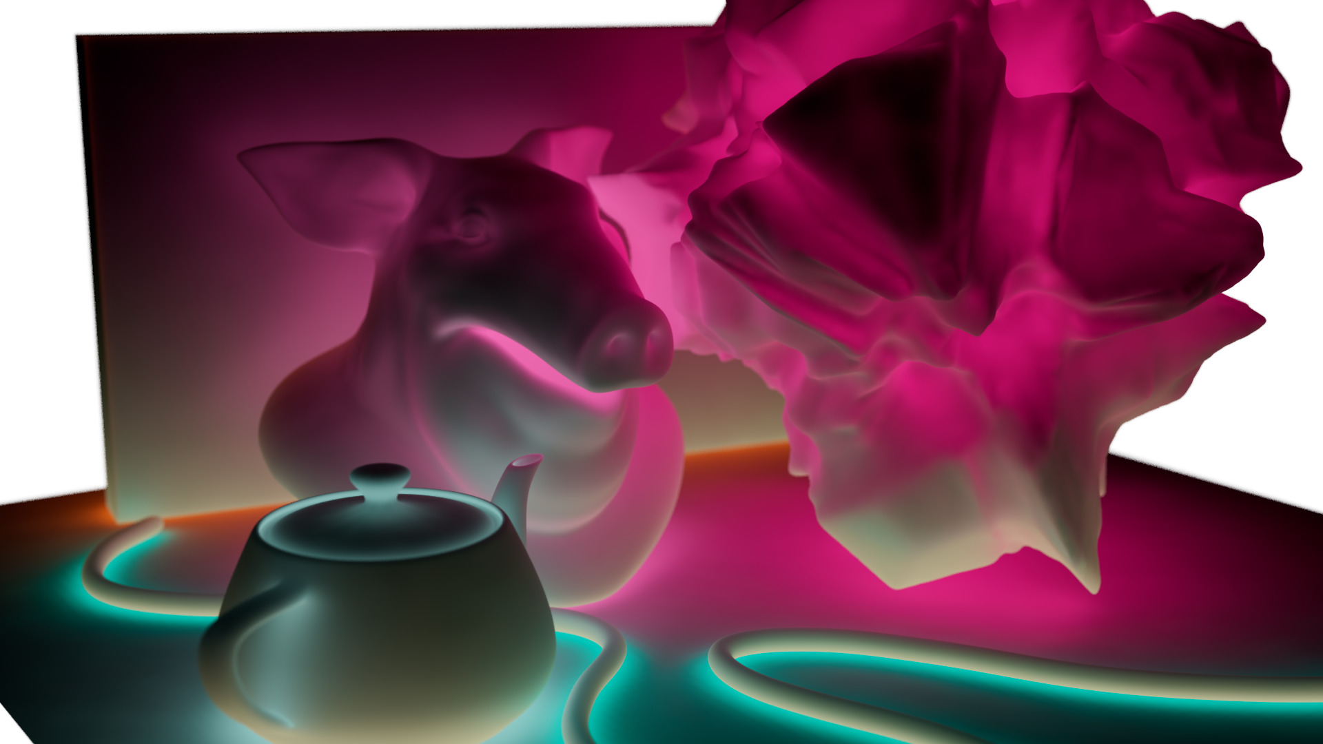
to sample any float or vector attribute in addition to measuring ray distance. Testing it with the Cd attribute results in some nice indirect color bleeding.

For the sim at the beginning of this post I used it to spread a temperature attribute inside a solver SOP. First the attribute is gathered towards the in- and outside via ray sampling and their radiant flux accumulated (using the gathered temperature as T_h and the initial temp as T_c in the formula below). The asset’s ‘incidence angle’ weight is used to introduce the Lambert-Cosine-Law. As a final step the dissipating heat Q is calculated and subtracted

Q = \sigma(T_h^4-T_c^4)A
• \sigma=Stefan Boltzmann constant
• A=Area
• T_c = ambient Temp
• T_h = reference Temp (at temp 1.0)

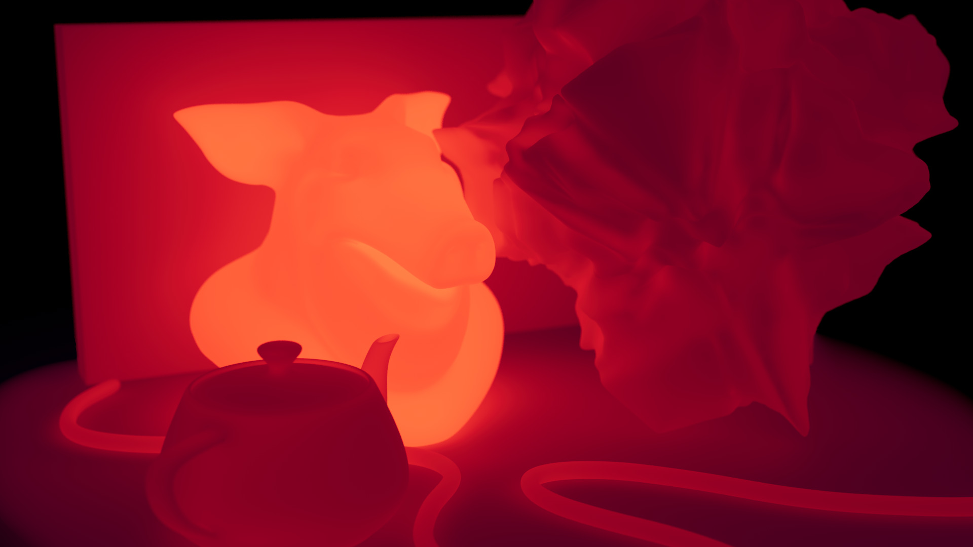
Since the sampling is limited to surfaces the heat kinda gets ‘stuck’ in high curvature areas. Maybe I’ll add an option for ray marching to improve this.